这种分析貌似在大模型时代没有使用那么多了,所以这里大概了解一下.
主要了解CAM,Grad-CAM可视化方法以及Sillancy map的概念
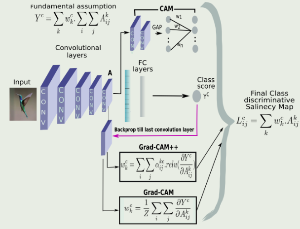
Learning Deep Features for Discriminative Localization
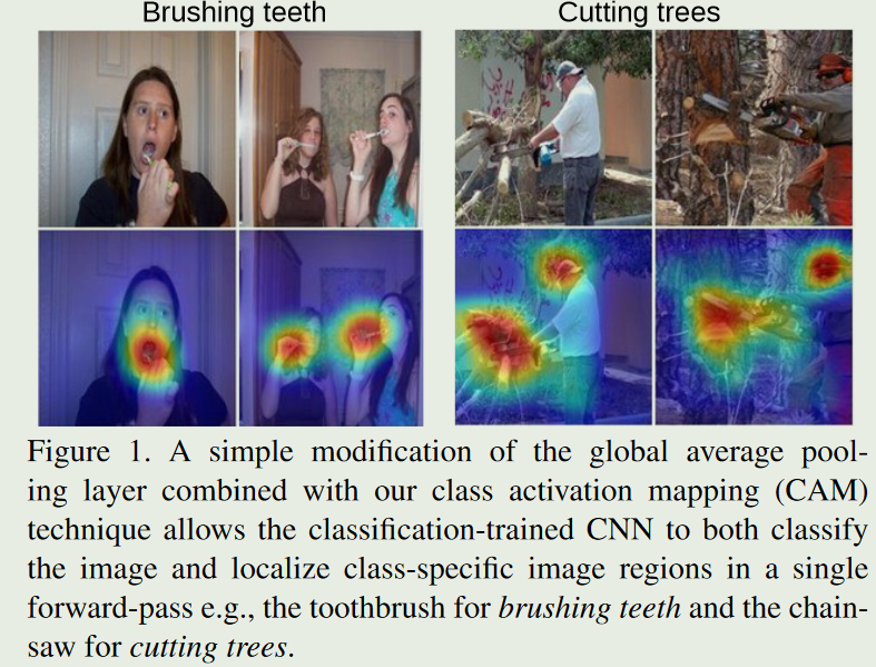
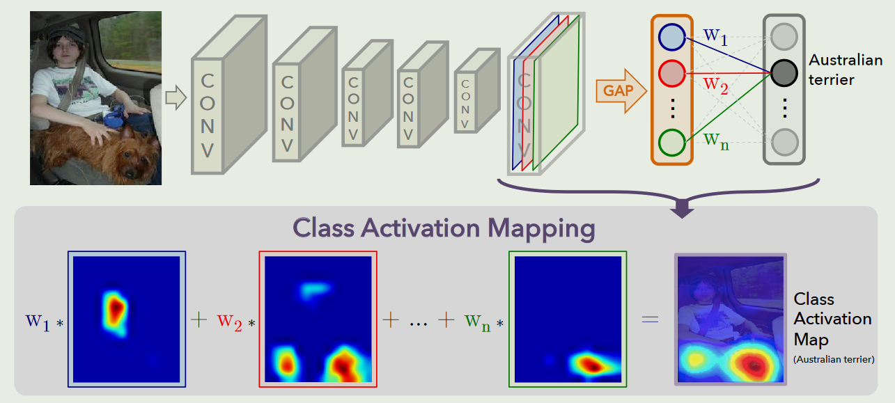
对于给定的图像,令f~k~( x , y)表示空间位置( x , y)处最后一个卷积层中单元k的激活值.然后,对于单元k,执行全局平均池化的结果F^k^为∑~x,y~ f~k~( x ,y).因此,对于给定的类c,softmax的输入S~c~=∑~k~ w^c^ ~k~F~k~,其中w^c^~k~是单位k对应于类c的权重.本质上,w^c^~k~表示F~k~对c类的重要性.
最后通过exp(S~c~ )/∑~c~ exp(S~c~ )给出类c,P~c~的softmax的输出.
通过将F~k~ =∑~x,y~f~k~( x,y)插入类得分S~c~,得到
将M~c~定义为c类的类激活映射,其中每个空间元素由S~c~ =∑~x,y~M~c~( x ,y),因此M~c~( x , y)直接表明空间网格( x , y)上的激活导致图像分类到c类的重要性.
所以这里的class activation map是根据卷积层特征来的,权重值计算依赖于global pooling.
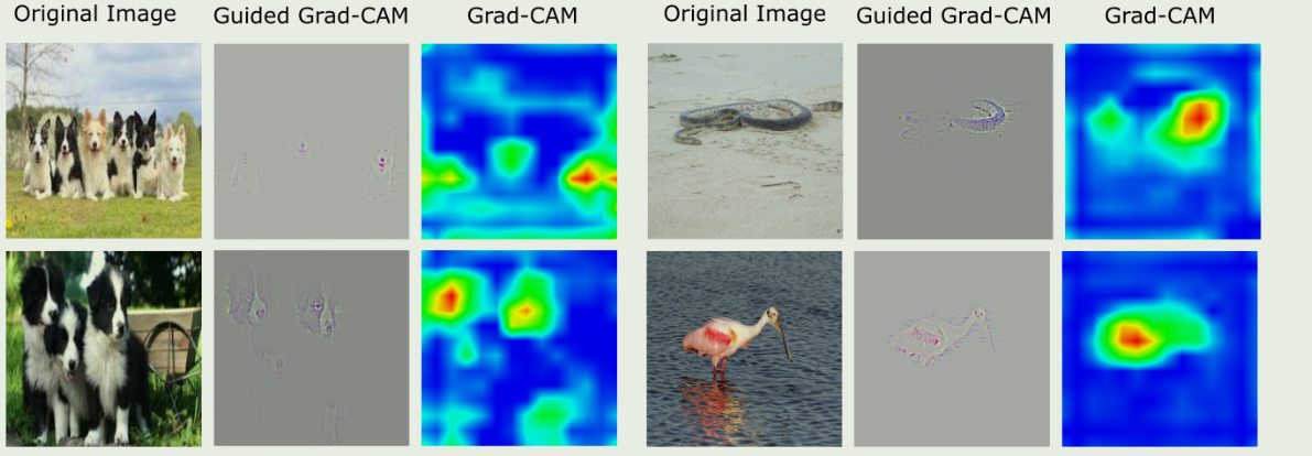
Grad-CAM: Visual Explanations from Deep Networks via Gradient-based Localization
CAM对于网络结构有要求,不采用GAP方法不能使用;且只能可视化最后一层的卷积
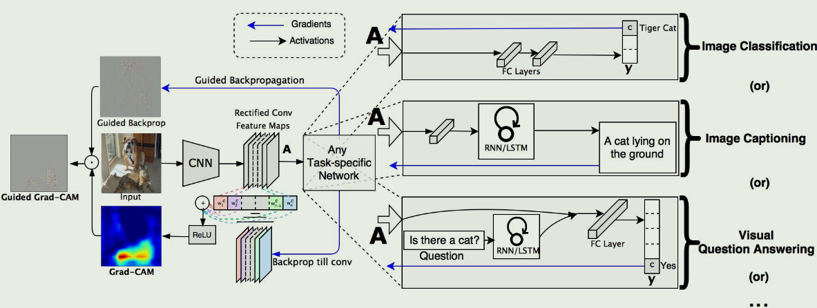
提出了一种从基于卷积神经网络( Convolutional Neural Network,CNN )的一大类模型中为决策产生”视觉解释”的技术,使其更加透明和可解释.
我们的方法- -梯度加权类激活映射( Gradient-weighted Class Activation Mapping,Grad-CAM ),利用任意目标概念(在分类网络中说’狗’ ,或者在描述网络中说词序列)流入最终卷积层的梯度,产生一个粗略的定位图,突出图像中的重要区域,用于预测概念
与以前的方法不同,Grad - CAM适用于各种各样的CNN模型家族:( 1 )具有全连接层的CNN (例如. VGG ),( 2 )用于结构化输出的CNNs (如字幕),( 3 )用于具有多模态输入(例如,视觉问答)或强化学习的任务的CNNs,都没有架构变化或重新训练.
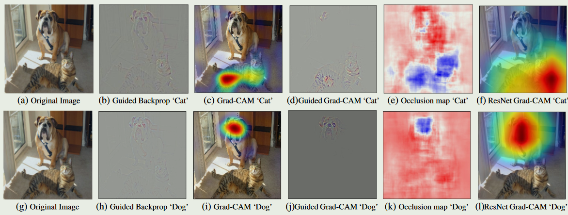
其中A^k^是特征图的值,权重由自己定变成了梯度.
为了得到对任意类c的宽u和高v的类判别局部化映射Grad - CAM Lc Grad-CAM∈R^u×v^,我们首先计算类c的得分y~c~ (在softmax之前)关于卷积层的特征图激活A~k~的梯度,即∑y~c~∑A~k~。
Grad-CAM++: Generalized Gradient-based Visual Explanations for Deep Convolutional Networks
本文的工作主要受到两种算法的启发,即CAM和Grad-CAM,这两种算法在当今被广泛使用.
CAM和Grad-CAM都基于一个基本假设,即对于特定类别c的最终得分Y~c~可以写成其全局平均池化最后一个卷积层特征图A~k~的线性组合
在Grad - CAM和CAM中基于梯度的可视化技术的基础上提出了一种广义的方法,称为Grad - CAM + +,它是通过显式地建模CNN特征图中每个像素对最终输出的贡献来制定的。
Smooth Grad-CAM++: An Enhanced Inference Level Visualization Technique for Deep Convolutional Neural Network Models
加入噪声
由于添加了噪声,所以更能够突出特征图在噪声中robust的部分,这部分被认为更重要;此方法可以用来比较图片不同位置对神经元的激活强度,所以可以进行choosing neurons的操作
Saliency map
Visualizing Neural Networks using Saliency Maps in PyTorch | by Aditya Rastogi | DataDrivenInvestor
表示显著性.1
2
3
4
5
6
7
8
9
10
11
12
13
14
15
16
17
18
19
20
21
22
23
24
25
26
27
28
29
30
31
32
33
34
35
36
37
38
39
40
41
42
43
44def normalize(image):
return (image - image.min()) / (image.max() - image.min())
# return torch.log(image)/torch.log(image.max())
def compute_saliency_maps(x, y, model):
model.eval()
x = x.cuda()
# we want the gradient of the input x
x.requires_grad_()
y_pred = model(x)
loss_func = torch.nn.CrossEntropyLoss()
loss = loss_func(y_pred, y.cuda())
loss.backward()
# saliencies = x.grad.abs().detach().cpu()
saliencies, _ = torch.max(x.grad.data.abs().detach().cpu(),dim=1)
# We need to normalize each image, because their gradients might vary in scale
saliencies = torch.stack([normalize(item) for item in saliencies])
return saliencies
# images, labels = train_set.getbatch(img_indices)
saliencies = compute_saliency_maps(images, labels, model)
# visualize
fig, axs = plt.subplots(2, len(img_indices), figsize=(15, 8))
for row, target in enumerate([images, saliencies]):
for column, img in enumerate(target):
if row==0:
axs[row][column].imshow(img.permute(1, 2, 0).numpy())
# What is permute?
# In pytorch, the meaning of each dimension of image tensor is (channels, height, width)
# In matplotlib, the meaning of each dimension of image tensor is (height, width, channels)
# permute is a tool for permuting dimensions of tensors
# For example, img.permute(1, 2, 0) means that,
# - 0 dimension is the 1 dimension of the original tensor, which is height
# - 1 dimension is the 2 dimension of the original tensor, which is width
# - 2 dimension is the 0 dimension of the original tensor, which is channels
else:
axs[row][column].imshow(img.numpy(), cmap=plt.cm.hot)
plt.show()
plt.close()
Smooth Grad
https://arxiv.org/pdf/1706.03825.pdf
Smooth grad 的方法是,在圖片中隨機地加入 noise,然後得到不同的 heatmap,把這些 heatmap 平均起來就得到一個比較能抵抗 noisy gradient 的結果
1 | # Smooth grad |
简单来说,就是执行多个epoch然后每次添加一个噪声进行forward(注意噪声也带梯度),每次将计算损失并将梯度累加,最后归一化
Filter Explaination
Deep Dream: Visualizing the features learnt by Convolutional Networks in PyTorch (reurl.cc)
通过hook得到卷积层的结果进行可视化.1
2
3
4
5
6
7
8
9
10
11
12
13
14
15
16
17
18
19
20
21
22
23
24
25
26
27
28
29
30
31
32
33
34
35
36
37
38
39
40
41
42
43
44
45
46
47
48
49
50
51
52def normalize(image):
return (image - image.min()) / (image.max() - image.min())
layer_activations = None
def filter_explanation(x, model, cnnid, filterid, iteration=100, lr=1):
# x: input image
# cnnid: cnn layer id
# filterid: which filter
model.eval()
def hook(model, input, output):
global layer_activations
layer_activations = output
hook_handle = model.cnn[cnnid].register_forward_hook(hook)
# When the model forwards through the layer[cnnid], it needs to call the hook function first
# The hook function save the output of the layer[cnnid]
# After forwarding, we'll have the loss and the layer activation
# Filter activation: x passing the filter will generate the activation map
model(x.cuda()) # forward
# Based on the filterid given by the function argument, pick up the specific filter's activation map
# We just need to plot it, so we can detach from graph and save as cpu tensor
filter_activations = layer_activations[:, filterid, :, :].detach().cpu()
# Filter visualization: find the image that can activate the filter the most
x = x.cuda()
x.requires_grad_()
# input image gradient
optimizer = Adam([x], lr=lr)
# Use optimizer to modify the input image to amplify filter activation
for iter in range(iteration):
optimizer.zero_grad()
model(x)
objective = -layer_activations[:, filterid, :, :].sum()
# We want to maximize the filter activation's summation
# So we add a negative sign
objective.backward()
# Calculate the partial differential value of filter activation to input image
optimizer.step()
# Modify input image to maximize filter activation
filter_visualizations = x.detach().cpu().squeeze()
# Don't forget to remove the hook
hook_handle.remove()
# The hook will exist after the model register it, so you have to remove it after used
# Just register a new hook if you want to use it
return filter_activations, filter_visualizations1
2
3
4
5
6
7
8
9
10
11
12
13
14images, labels = train_set.getbatch(img_indices)
filter_activations, filter_visualizations = filter_explanation(images, model, cnnid=6, filterid=0, iteration=100, lr=0.1)
fig, axs = plt.subplots(3, len(img_indices), figsize=(15, 8))
for i, img in enumerate(images):
axs[0][i].imshow(img.permute(1, 2, 0))
# Plot filter activations
for i, img in enumerate(filter_activations):
axs[1][i].imshow(normalize(img))
# Plot filter visualization
for i, img in enumerate(filter_visualizations):
axs[2][i].imshow(normalize(img.permute(1, 2, 0)))
plt.show()
plt.close()
filter_activations就是卷积层的权重,通过hook得到filter_activations = layer_activations[:, filterid, :, :].detach().cpu()
register_forward_hook可以修改输出,修改输入不会对forward过程产生作用.
register_full_backward_hook可以修改grad_input对应于输入(在forward时)的梯度(反向传播时的输入梯度就是需要计算的梯度)
filter_visualizations是输入数据带上梯度,通过多个epoch计算损失函数(-layer_activations[:, filterid, :, :].sum()),使得激活值更大.
Integrated Gradients
根据代码看下来,就是在图像上不断加噪声,看起来跟积分类似,然后计算梯度加起来.
1 | class IntegratedGradients(): |
1 | # put the image to cuda |
